Orbitals, Fermions and Gradients: Getting started with Tequila

pip install git+https://github.com/aspuru-guzik-group/tequila.git

Slides in notebook form: github.com/kottmanj/talks_and_material

In [2]:
import tequila as tq
import numpy

Warmup:

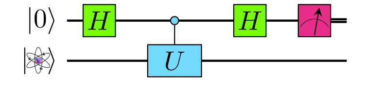
Original idea for quantum computers: Simulate nature

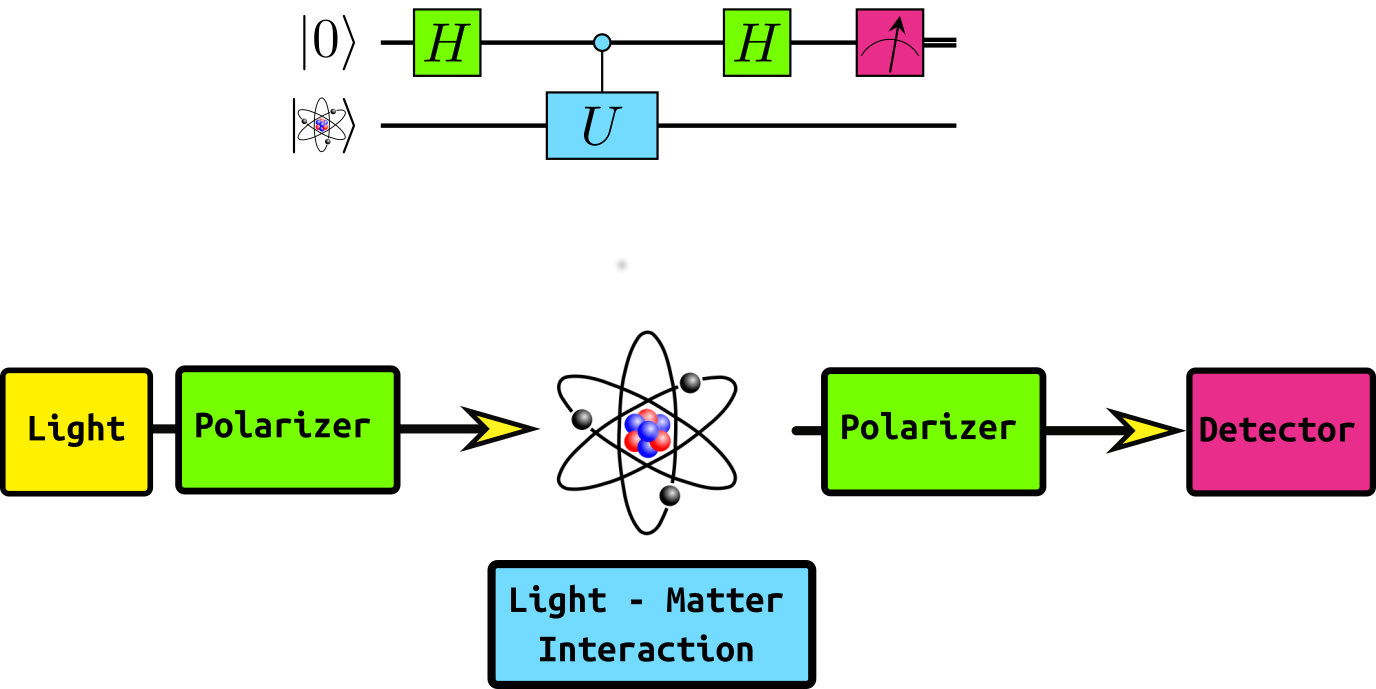
Assume: $U = e^{i\frac{\theta}{2}G}$ with hermitian matrix $G$ and $\theta=2\pi$.
For simplicity: Assume eigenvalues of $G$ are $0$ and $1$

Concrete example: $$ G = \sigma_x + 1 $$

In [3]:
G = 0.5*(tq.paulis.X(1)+1.0)
In [4]:
val, vec = numpy.linalg.eigh(G.to_matrix())
eigenstates = []
for i in range(2):
    wfn = tq.QubitWaveFunction.from_array(vec[:,i])
    print("energy = {:+2.5f}, wfn=".format(val[i]), wfn)
    eigenstates.append(wfn)
energy = +0.00000, wfn= -0.7071|0> +0.7071|1> 
energy = +1.00000, wfn= +0.7071|0> +0.7071|1> 

Simulated Laboratory

In [5]:
a=2*numpy.pi
cU = tq.gates.Trotterized(generator=G, angle=a, control=0)
U = tq.gates.H(0) + cU + tq.gates.H(0)
wfn = tq.simulate(U)
print("wavefunction after circuit:\n", wfn)
wavefunction after circuit:
 +0.5000e^(-0.2500Ï€i)|00> +0.5000e^(-0.2500Ï€i)|10> +0.5000e^(+0.7500Ï€i)|01> +0.5000e^(-0.2500Ï€i)|11> 
In [53]:
Qp = tq.paulis.Qp(0) # Qp = |0><0| = 0.5(Z+1)
wfn2 = Qp(wfn)
wfn2 = wfn2.normalize()
print("wavefunction after measurements:\n",wfn2)
fidelity = numpy.abs(wfn2.inner(eigenstates[0]))**2
print("fidelity with eigenstate 0:", fidelity )
wavefunction after measurements:
 +0.7071e^(-0.2500Ï€i)|00> +0.7071e^(+0.7500Ï€i)|01> 
fidelity with eigenstate 0: 0.9999999999999998

A Toy VQE

Example before: Quantum Phase Estimation (measure eigenvalues of Hermitian operator)

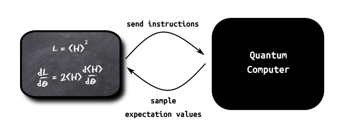
Now: Variational Quantum Eigensolver (minimize expectation value of Hermitian operator)

$$ \min_{\theta} \langle H \rangle_{U(\theta)} $$
In [7]:
H = 0.5*(tq.paulis.X(0) + 1.0)
U = tq.gates.Ry(target=0, angle="a")
E = tq.ExpectationValue(H=H, U=U)
In [8]:
result = tq.minimize(E)
WARNING:absl:No GPU/TPU found, falling back to CPU. (Set TF_CPP_MIN_LOG_LEVEL=0 and rerun for more info.)
Optimizer: <class 'tequila.optimizers.optimizer_scipy.OptimizerSciPy'> 
backend         : qulacs
device          : None
samples         : None
save_history    : True
noise           : None

Method          : BFGS
Objective       : 1 expectationvalues
gradient        : 2 expectationvalues

active variables : 1

E=+0.50000000  angles= {a: 0.0}  samples= None
E=+0.26028723  angles= {a: -0.5}  samples= None
E=+0.00026787  angles= {a: -1.6035311193256832}  samples= None
E=+0.00001204  angles= {a: -1.5638552774723973}  samples= None
E=+0.00000000  angles= {a: -1.5707973321904534}  samples= None
Optimization terminated successfully.
         Current function value: 0.000000
         Iterations: 4
         Function evaluations: 5
         Gradient evaluations: 5

Simulate and Compile Objectives

In [9]:
# simulate objectives
energy1 = tq.simulate(E, variables={"a": -numpy.pi/2})
# compile objectives and use as functions
f = tq.compile(E)
energy2 = f({"a":-numpy.pi/2})
# use different backends and options
energy3 = tq.simulate(E, variables={"a": -numpy.pi/2}, backend="cirq", samples=1000)

Beyond Groundstates

Overlap punishment:

$$ S^2\left(\phi, \psi\right)= \lvert\langle \phi \vert \psi \rangle\rvert^2 = \langle Q_+ \rangle_{U_\phi^\dagger U_{\psi}} , \quad Q_+ = \lvert 00\dots0 \rangle\langle 00\dots0 \lvert$$

In [10]:
Uex = tq.gates.Ry(angle="b", target=0)
S2 = tq.ExpectationValue(H=tq.paulis.Qp(0), U=Uex+U.dagger())
opt_gs = {"a":-0.5*numpy.pi}
L = tq.ExpectationValue(H=H, U=Uex) + 10.0*S2
In [11]:
result_ex = tq.minimize(L, 
                        initial_values=opt_gs, 
                        variables=["b"])
 /home/jsk/projects/OpenVQE/src/tequila/optimizers/optimizer_base.py:422: TequilaWarning:initial_variables given but not complete: Autocompleted with zeroes
Optimizer: <class 'tequila.optimizers.optimizer_scipy.OptimizerSciPy'> 
backend         : qulacs
device          : None
samples         : None
save_history    : True
noise           : None

Method          : BFGS
Objective       : 2 expectationvalues
gradient        : 6 expectationvalues

active variables : 1

E=+5.49999475  angles= {b: 0.0, a: -1.5707973321904534}  samples= None
E=+1.68925405  angles= {b: 1.01, a: -1.5707973321904534}  samples= None
E=+1.75247025  angles= {b: 2.157473194149607, a: -1.5707973321904534}  samples= None
E=+1.00000119  angles= {b: 1.5700696738344724, a: -1.5707973321904534}  samples= None
E=+1.00000000  angles= {b: 1.5708347830881644, a: -1.5707973321904534}  samples= None
Optimization terminated successfully.
         Current function value: 1.000000
         Iterations: 3
         Function evaluations: 5
         Gradient evaluations: 5

In [12]:
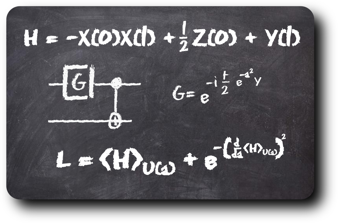
a = tq.Variable("a")
angle = (-a**2).apply(tq.numpy.exp)
U = tq.gates.Ry(angle=angle*numpy.pi, target=0)
U += tq.gates.X(target=1, control=0)
H = tq.QubitHamiltonian("-1.0X(0)X(1)+0.5Z(0)+Y(1)")
E = tq.ExpectationValue(H=H, U=U)
dE = tq.grad(E, "a")
objective = E + (-(dE**2)).apply(tq.numpy.exp)
f = tq.compile(objective)
In [13]:
import matplotlib.pyplot as plt
start=-2.0
stop=2.0
values = {}
for value in [start + i/100*(stop-start) for i in range(100)]:
    values[value] = f({"a":value})
plt.plot(list(values.keys()), list(values.values()))
plt.show()

In [14]:
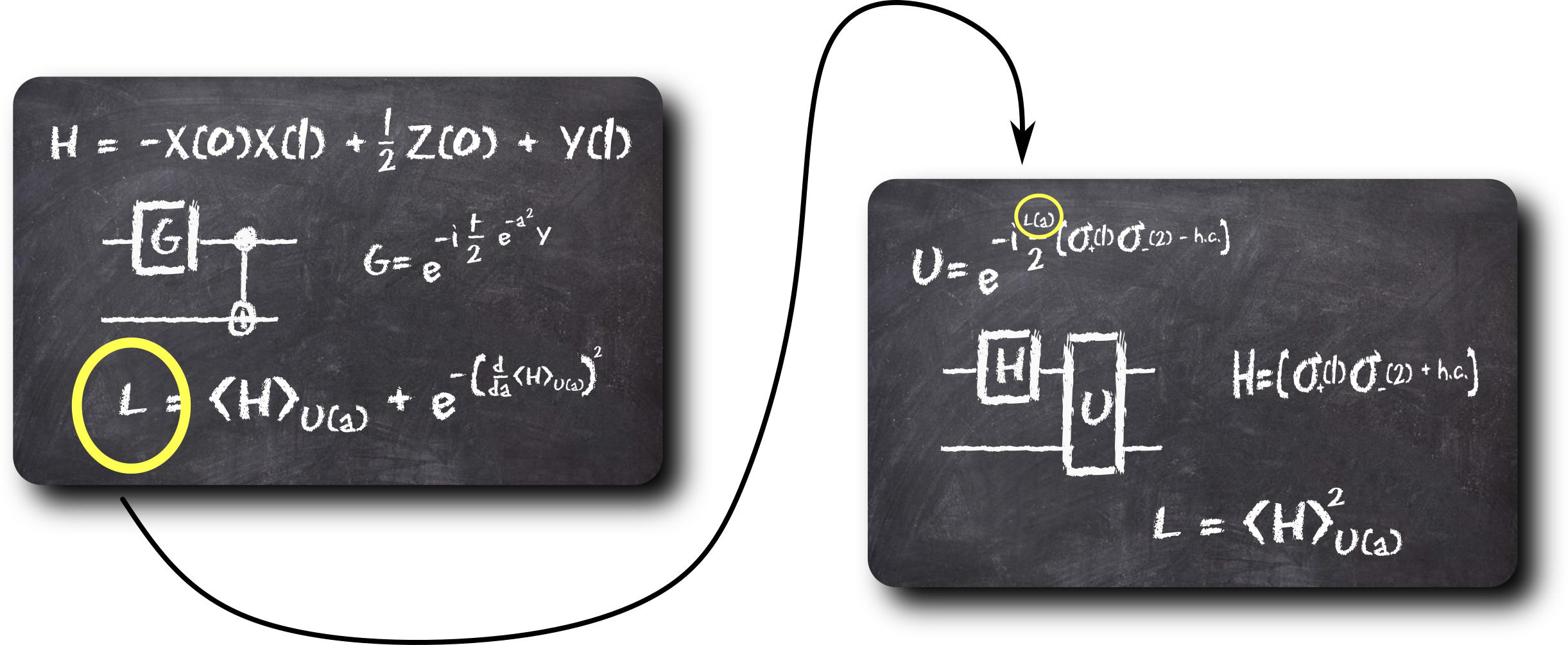
H =  tq.paulis.Sp(0)*tq.paulis.Sm(1)
H += tq.paulis.Sm(0)*tq.paulis.Sp(1)
U =  tq.gates.X(0)
U += tq.gates.QubitExcitation(angle=f, target=[0,1])
L2 = tq.ExpectationValue(H=H, U=U)**2
f2 = tq.compile(L2)
In [15]:
import matplotlib.pyplot as plt
start=-2.0
stop=2.0
steps=100
values = {}
for value in [start + i/steps*(stop-start) for i in range(steps)]:
    values[value] = f2({"a":value})
plt.plot(list(values.keys()), list(values.values()))
plt.show()

Example: Meta-VQE

A. Cervera-Lierta, JSK, A. Aspuru-Guzik, ArXiv:2009.13545

Learn the relation of a parameters in the Hamiltonian and in the circuit
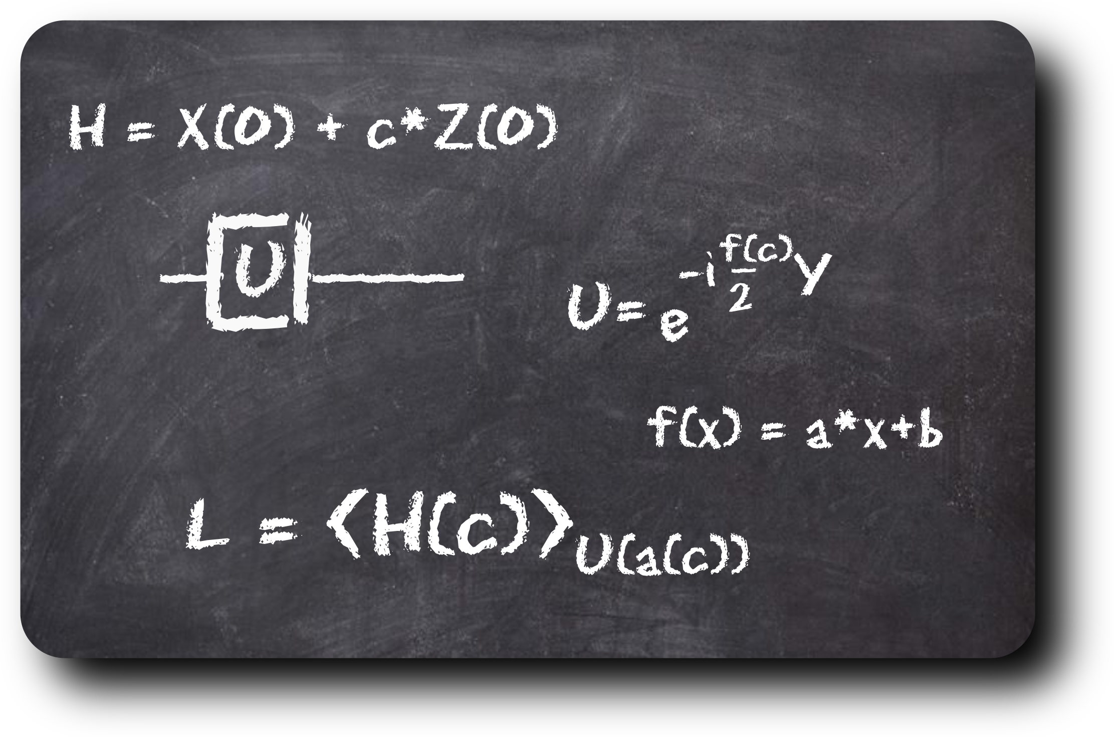
In [16]:
def meta_angle(x):
    a = tq.assign_variable("a")
    b = tq.assign_variable("b")
    return x*a-b

def make_H(x):
    return tq.paulis.X(0) + x*tq.paulis.Z(0)

def make_U(angle):
    angle = tq.assign_variable(angle)
    return tq.gates.Ry(target=0, angle=angle*numpy.pi)

Training

In [17]:
training_points = [0.0, 0.5, 1.0]
meta_objective = 0.0
for x in training_points:
    meta_objective += tq.ExpectationValue(H=make_H(x), U=make_U(meta_angle(x)))

meta_objective = 1.0/len(training_points)*meta_objective
In [18]:
meta_vqe_result = tq.minimize(meta_objective)
Optimizer: <class 'tequila.optimizers.optimizer_scipy.OptimizerSciPy'> 
backend         : qulacs
device          : None
samples         : None
save_history    : True
noise           : None

Method          : BFGS
Objective       : 3 expectationvalues
gradient        : 18 expectationvalues

active variables : 2

E=+0.50000000  angles= {a: 0.0, b: 0.0}  samples= None
E=+0.03163936  angles= {a: -0.45168573145495755, b: 0.9033714629099151}  samples= None
E=-1.10308790  angles= {a: -0.20895075848145425, b: 0.4179015169629085}  samples= None
E=-0.60310841  angles= {a: -0.5721265537434792, b: 0.6376424028446308}  samples= None
E=-1.17348516  angles= {a: -0.29224800825863895, b: 0.468300832380787}  samples= None
E=-1.17658091  angles= {a: -0.23413025767017326, b: 0.518145642557484}  samples= None
E=-1.17678094  angles= {a: -0.24759858034771412, b: 0.5085406576584631}  samples= None
Optimization terminated successfully.
         Current function value: -1.176781
         Iterations: 4
         Function evaluations: 7
         Gradient evaluations: 7

Testing

In [19]:
test_points=[0.0 + x/100 for x in range(100)]
predicted_angles = {}
opt_angles = {}
for x in test_points:
    predicted = meta_angle(x)(variables=meta_vqe_result.variables)
    predicted_angles[x] = predicted
    objective = tq.ExpectationValue(H=make_H(x), U=make_U("x"))
    opt = tq.minimize(objective, silent=True, initial_values=predicted)
    opt_angles[x] = opt.variables["x"]
In [20]:
plt.plot(list(predicted_angles.keys()), list(predicted_angles.values()), label="predicted", marker="o", markersize=5)
plt.plot(list(opt_angles.keys()), list(opt_angles.values()), label="opt", marker="x", markersize=3)
plt.legend()
plt.show()
In [21]:
def meta_angle(x):
    a = tq.assign_variable("a")
    b = tq.assign_variable("b")
    c = tq.assign_variable("c")
    d = tq.assign_variable("d")
    return b*x**2 + c*x + d
In [23]:
plt.figure()
plt.plot(list(predicted_angles.keys()), list(predicted_angles.values()), label="predicted", marker="o", markersize=5)
plt.plot(list(opt_angles.keys()), list(opt_angles.values()), label="opt", marker="x", markersize=3)
plt.legend()
plt.show()

Example: Quantum Chemistry
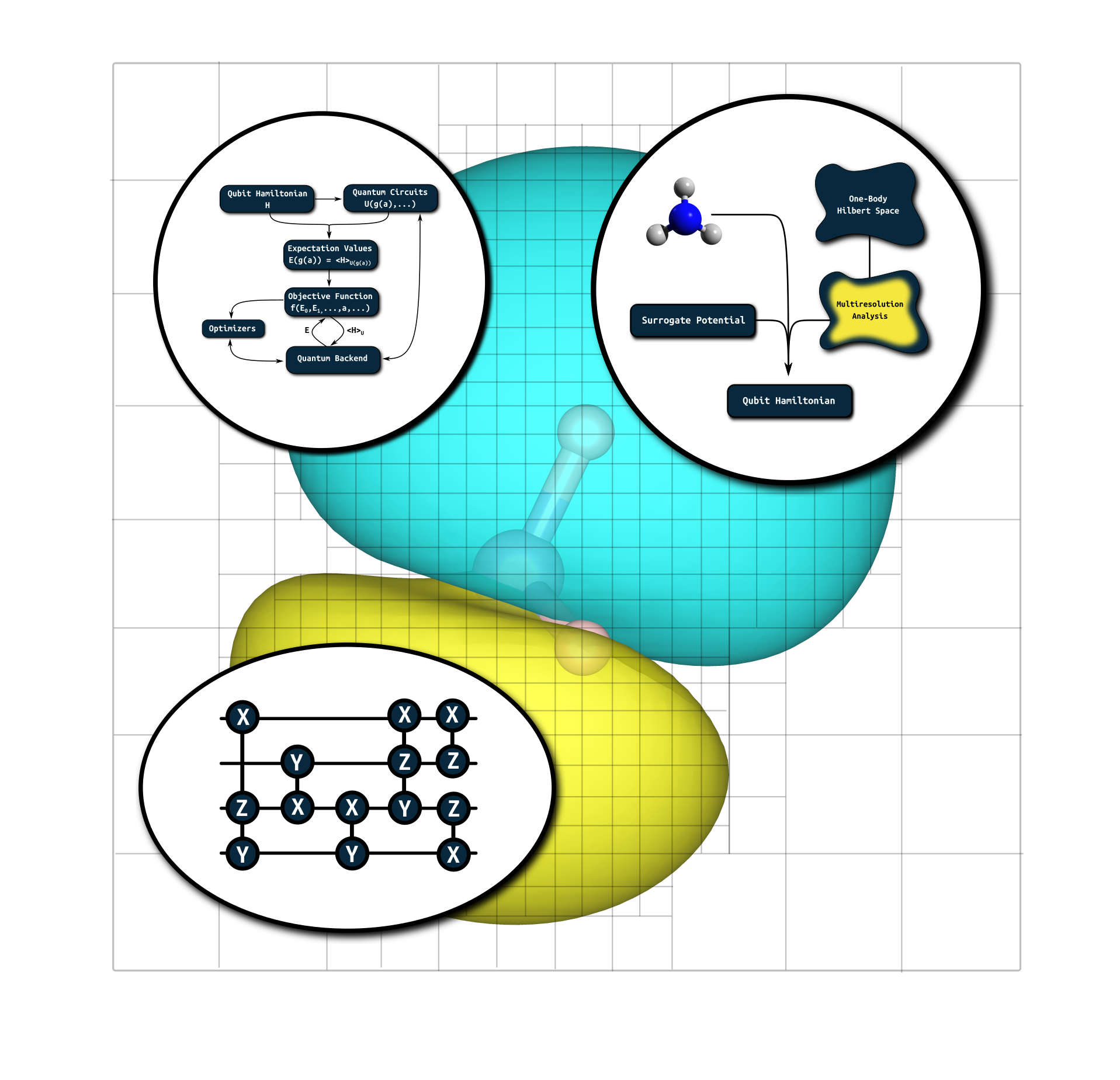
Dependencies

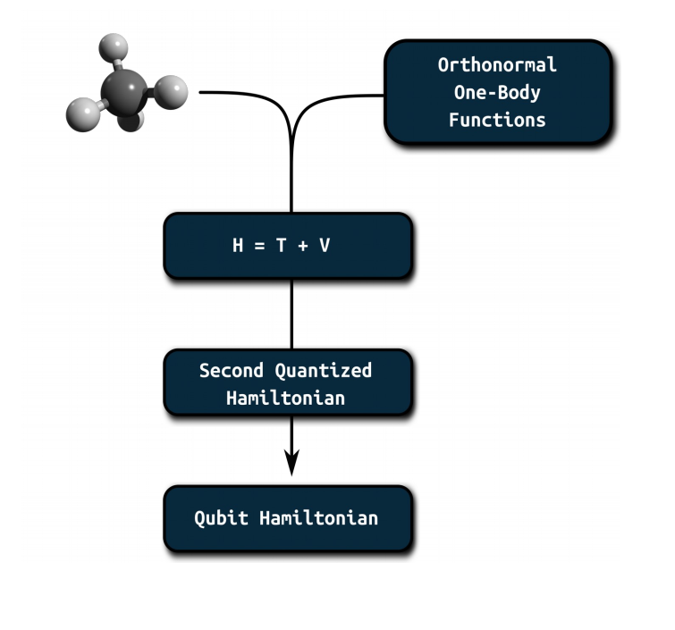
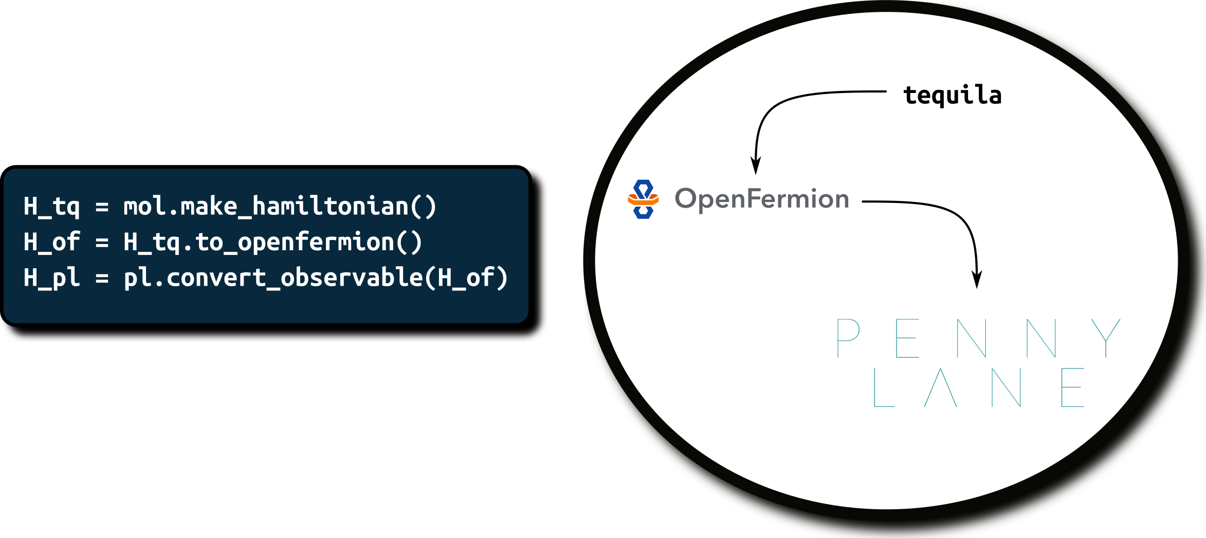
Molecular Hamiltonian in Qubit Representation

In [25]:
geomstring = "H 0.0 0.0 0.0\nH 0.0 0.0 {R}".format(R=0.7)
mol = tq.Molecule(geometry=geomstring,basis_set="sto-3g")
H = mol.make_hamiltonian()
In [26]:
print(H)
-0.0421+0.1777Z(0)+0.1777Z(1)-0.2427Z(2)-0.2427Z(3)+0.1706Z(0)Z(1)+0.0448Y(0)X(1)X(2)Y(3)-0.0448Y(0)Y(1)X(2)X(3)-0.0448X(0)X(1)Y(2)Y(3)+0.0448X(0)Y(1)Y(2)X(3)+0.1229Z(0)Z(2)+0.1677Z(0)Z(3)+0.1677Z(1)Z(2)+0.1229Z(1)Z(3)+0.1763Z(2)Z(3)

Hartree-Fock Reference State

In [27]:
U = mol.prepare_reference()
E = tq.ExpectationValue(H=H, U=U)
hf_energy = tq.simulate(E)
print("EHF = {:+2.5f}".format(hf_energy))
EHF = -1.11735
In [28]:
print(E)
Objective with 1 unique expectation values
total measurements = 15
variables          = []
types              = not compiled
In [29]:
E = tq.ExpectationValue(H=H, U=U, optimize_measurements=True)
print(tq.compile(E, backend="qiskit"))
Objective with 2 unique expectation values
total measurements = 2
variables          = []
types              = [<class 'tequila.simulators.simulator_qiskit.BackendExpectationValueQiskit'>]
In [54]:
geomstring = "H 0.0 0.0 0.0\nLi 0.0 0.0 {R}".format(R=0.7)
mol = tq.Molecule(geometry=geomstring, basis_set="sto-3g",
                  transformation="BravyiKitaev")
print(mol)
<class 'tequila.quantumchemistry.psi4_interface.QuantumChemistryPsi4'>
Qubit Encoding
transformation=<function bravyi_kitaev at 0x7f418cdffa70>

Parameters
basis_set       : sto-3g          
geometry        : H 0.0 0.0 0.0
Li 0.0 0.0 0.7 
description     :                 
multiplicity    : 1               
charge          : 0               
closed_shell    : True            
name            : molecule        

Psi4 Data
Point Group (full) : c_inf_v         
Point Group (used) : c2v             
nirrep          : 4 
irreps          : ['A1', 'A2', 'B1', 'B2'] 
mos per irrep   : [4, 0, 1, 1]    

Orbitals:
0 : 0A1 energy = -2.519793 
1 : 1A1 energy = -0.296569 
2 : 2A1 energy = +0.057778 
3 : 0B1 energy = +0.139822 
4 : 0B2 energy = +0.139822 
5 : 3A1 energy = +0.599617 

Active Spaces

In [31]:
geomstring = "H 0.0 0.0 0.0\nLi 0.0 0.0 {R}".format(R=0.7)
active={"A1":[1,2]}
mol = tq.Molecule(geometry=geomstring,
                  basis_set="sto-3g",
                  active_orbitals=active)
H = mol.make_hamiltonian()

Manually Construct an Ansatz

In [32]:
U = tq.gates.Ry(angle="a", target=0)
U += tq.gates.X(1)
U += tq.gates.X(target=1, control=0)
U += tq.gates.X(target=2, control=1)
U += tq.gates.X(target=3, control=2)
U += tq.gates.X(target=1)
In [33]:
tq.draw(U)

Optimize the Ansatz

In [34]:
E = tq.ExpectationValue(H=H, U=U)
result = tq.minimize(E)
energy_np = numpy.linalg.eigvalsh(H.to_matrix())[0]
energy_fci = mol.compute_energy("fci")
Optimizer: <class 'tequila.optimizers.optimizer_scipy.OptimizerSciPy'> 
backend         : qulacs
device          : None
samples         : None
save_history    : True
noise           : None

Method          : BFGS
Objective       : 1 expectationvalues
gradient        : 2 expectationvalues

active variables : 1

E=-6.95631152  angles= {a: 0.0}  samples= None
E=-6.95641192  angles= {a: -0.009415864944458008}  samples= None
E=-6.95704807  angles= {a: -0.04707932472229004}  samples= None
E=-6.96332136  angles= {a: -0.19773316383361816}  samples= None
E=-7.04345170  angles= {a: -0.8003485202789307}  samples= None
E=-7.48465953  angles= {a: -3.2108099460601807}  samples= None
E=-7.48119139  angles= {a: -2.913032986993547}  samples= None
E=-7.48611221  angles= {a: -3.106200173015701}  samples= None
Optimization terminated successfully.
         Current function value: -7.486112
         Iterations: 1
         Function evaluations: 8
         Gradient evaluations: 8
In [35]:
print("VQE   = {:2.5f}".format(result.energy))
print("FCI   = {:2.5f}".format(energy_fci))
print("Numpy = {:2.5f}".format(energy_np))
VQE   = -7.48611
FCI   = -7.48612
Numpy = -7.48612

Manually construct an UCC ansatz

In [36]:
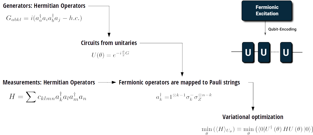
G0213 = mol.make_excitation_generator(indices=[(0,2),(1,3)])
Uex = tq.gates.Trotterized(generator=G0213, angle="a")
U = mol.prepare_reference() + Uex
In [37]:
tq.draw(U)
In [38]:
E = tq.ExpectationValue(H=H, U=U)
result = tq.minimize(E)
Optimizer: <class 'tequila.optimizers.optimizer_scipy.OptimizerSciPy'> 
backend         : qulacs
device          : None
samples         : None
save_history    : True
noise           : None

Method          : BFGS
Objective       : 1 expectationvalues
gradient        : 16 expectationvalues

active variables : 1

E=-7.48594487  angles= {a: 0.0}  samples= None
E=-7.48602179  angles= {a: 0.009415864944458008}  samples= None
E=-7.48611042  angles= {a: 0.031862458915351874}  samples= None
Optimization terminated successfully.
         Current function value: -7.486110
         Iterations: 2
         Function evaluations: 3
         Gradient evaluations: 3

Gradient Aware Construction

In [39]:
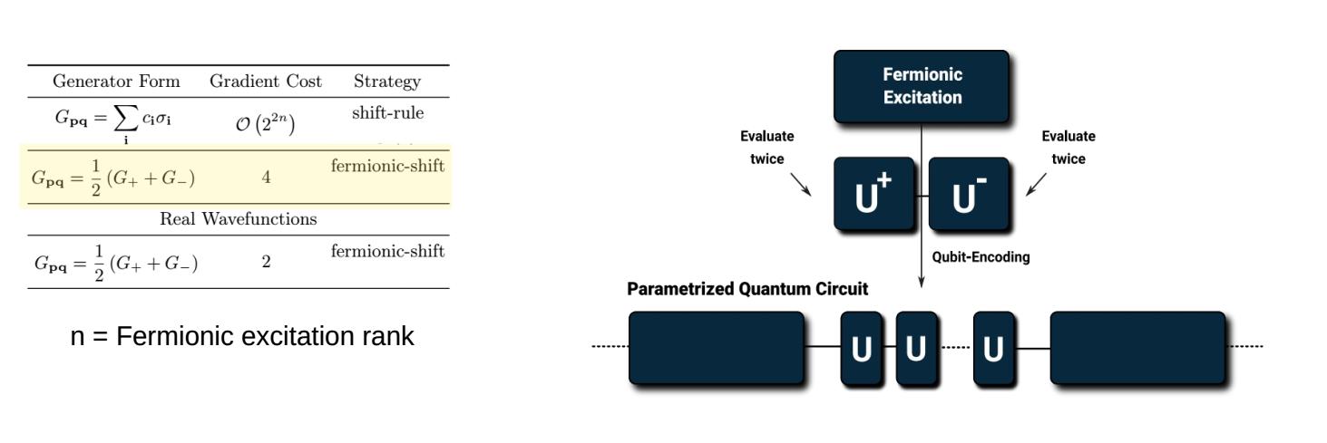
Uex = mol.make_excitation_gate([(0,2),(1,3)], "a")
U = mol.prepare_reference() + Uex
E = tq.ExpectationValue(H=H, U=U)
In [40]:
result = tq.minimize(E)
Optimizer: <class 'tequila.optimizers.optimizer_scipy.OptimizerSciPy'> 
backend         : qulacs
device          : None
samples         : None
save_history    : True
noise           : None

Method          : BFGS
Objective       : 1 expectationvalues
gradient        : 2 expectationvalues

active variables : 1

E=-7.48594487  angles= {a: 0.0}  samples= None
E=-7.48602179  angles= {a: 0.009415864944458008}  samples= None
E=-7.48611042  angles= {a: 0.031862458915351874}  samples= None
Optimization terminated successfully.
         Current function value: -7.486110
         Iterations: 2
         Function evaluations: 3
         Gradient evaluations: 3

Quantum Chemistry: Constructing the Hamiltonian

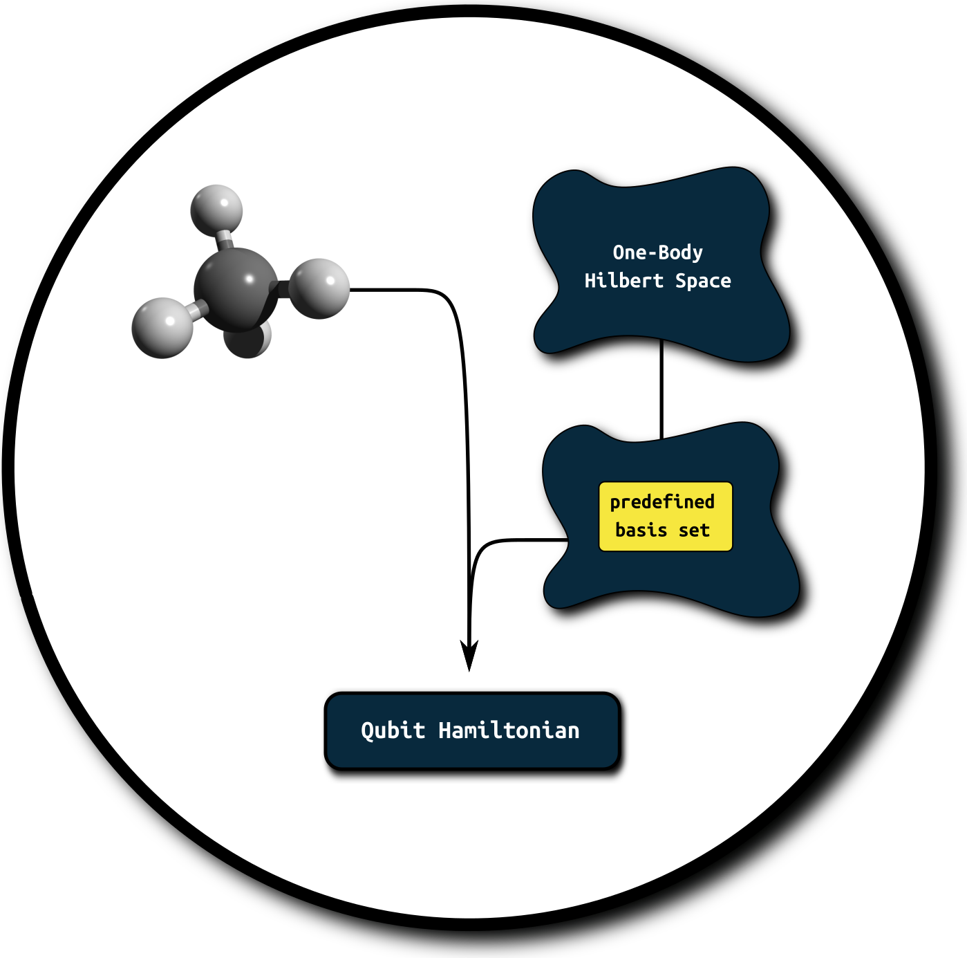
  • Well developed classical machinery
  • Unknown numerical error
  • Accurate results require large basis sets
  • High level of expertise required from the user

In [42]:
mol = tq.Molecule(geometry=geomstring, basis_set="cc-pVDZ")
print(mol.make_hamiltonian().n_qubits)
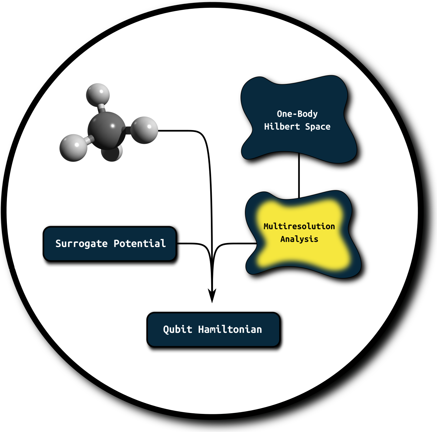
38

  • Basis-set-free
  • Physically interpretable limitations
  • Compact (save qubits)
  • Natural order on orbitals
  • Low level of expertise required from user
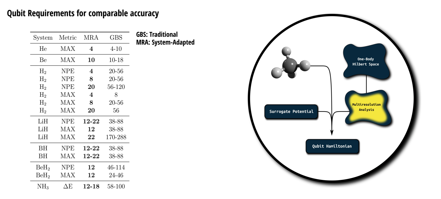
More

Basis-set-Free VQE:
JSK, P. Schleich, T. Tamayo-Mendoza, A. Aspuru-Guzik doi.org/10.1021/acs.jpclett.0c03410

Surrogate Model (PNO-MP2):
JSK, F. A. Bischoff, E. F. Valeev doi.org/10.1063/1.5141880

Tequila backend: Madness
R.J. Harrison et.al. doi.org/10.1137/15M1026171

MRA basics:
doi.org/10.18452/19357 (Chapter 2)

Review on classical applications:
F.A. Bischoff, doi.org/10.1016/bs.aiq.2019.04.003

In [7]:
mol = tq.Molecule(geometry="Li 0.0 0.0 0.0\nH 0.0 0.0 1.6", 
                  n_pno=4,
                  executable=madness_exe,
                  name="lih_1.6")
H = mol.make_hamiltonian()
U = mol.make_pno_upccgsd_ansatz(include_singles=False)
E = tq.ExpectationValue(H=H, U=U)
In [8]:
print(mol)
<class 'tequila.quantumchemistry.madness_interface.QuantumChemistryMadness'>
Qubit Encoding
transformation=<function jordan_wigner at 0x7f90eb2efa70>

Parameters
basis_set       : custom          
geometry        : Li 0.0 0.0 0.0
H 0.0 0.0 1.6 
description     :                 
multiplicity    : 1               
charge          : 0               
closed_shell    : True            
name            : lih_1.6         

MRA Orbitals    :
orbital 0, occupied reference orbital (0,), energy -2.44107 
orbital 1, occupied reference orbital (1,), energy -0.305942 
orbital 2, pno from pair (1, 1), MP2 occ 0.0113194 
orbital 3, pno from pair (1, 1), MP2 occ 0.00479669 
orbital 4, pno from pair (1, 1), MP2 occ 0.00479458 
orbital 5, pno from pair (1, 1), MP2 occ 0.00419803 

executable      : /home/jsk/devel/madness/build-opt//src/apps/pno/pno_integrals
htensor         : lih_1.6_htensor.npy
gtensor         : lih_1.6_gtensor.npy

In [75]:
result = tq.minimize(E)
Optimizer: <class 'tequila.optimizers.optimizer_scipy.OptimizerSciPy'> 
backend         : qulacs
device          : None
samples         : None
save_history    : True
noise           : None

Method          : BFGS
Objective       : 1 expectationvalues
gradient        : 8 expectationvalues

active variables : 4

E=-7.98721057  angles= {(0, ((2, 4), (3, 5)), None): 0.0, (0, ((2, 6), (3, 7)), None): 0.0, (0, ((2, 8), (3, 9)), None): 0.0, (0, ((2, 10), (3, 11)), None): 0.0}  samples= None
E=-8.01593186  angles= {(0, ((2, 4), (3, 5)), None): 0.12768793106079102, (0, ((2, 6), (3, 7)), None): 0.09198546409606934, (0, ((2, 8), (3, 9)), None): 0.09202122688293457, (0, ((2, 10), (3, 11)), None): 0.09455657005310059}  samples= None
E=-8.02032262  angles= {(0, ((2, 4), (3, 5)), None): 0.21350067509853055, (0, ((2, 6), (3, 7)), None): 0.14165840203560198, (0, ((2, 8), (3, 9)), None): 0.14177428603515832, (0, ((2, 10), (3, 11)), None): 0.13429117589170406}  samples= None
E=-8.02036286  angles= {(0, ((2, 4), (3, 5)), None): 0.2187140711919535, (0, ((2, 6), (3, 7)), None): 0.14006640996346112, (0, ((2, 8), (3, 9)), None): 0.1402723816504262, (0, ((2, 10), (3, 11)), None): 0.12927082915985516}  samples= None
E=-8.02037080  angles= {(0, ((2, 4), (3, 5)), None): 0.22235015051312715, (0, ((2, 6), (3, 7)), None): 0.13869881217448576, (0, ((2, 8), (3, 9)), None): 0.13896068272518608, (0, ((2, 10), (3, 11)), None): 0.12618000883095457}  samples= None
Optimization terminated successfully.
         Current function value: -8.020371
         Iterations: 4
         Function evaluations: 5
         Gradient evaluations: 5
final energy = -8.02037

Example: Adaptive Solvers

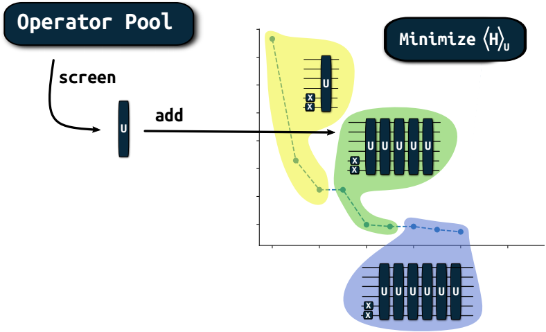
Original approaches:
Ryabynkin, Yen, Genin, Izmaylov, doi.org/10.1021/acs.jctc.8b00932
Grimsley, Economou, Barnes, Mayhall doi.org/10.1038/s41467-019-10988-2

Example: Adaptive Solvers

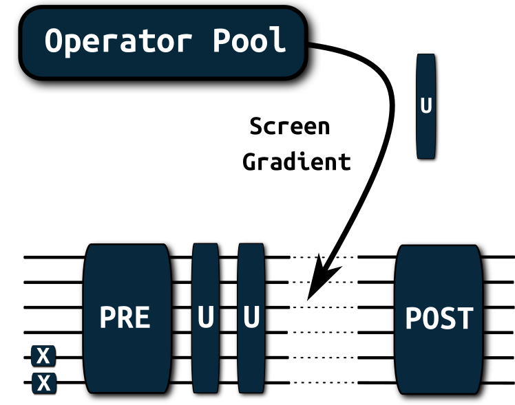
Tequila implementation:
JSK, Anand, Aspuru-Guzik. doi.org/10.1039/D0SC06627C

More examples on github

In [9]:
operator_pool = tq.apps.adapt.MolecularPool(molecule=mol, 
                                            indices="UpCCGSD")
solver = tq.apps.adapt.Adapt(operator_pool=operator_pool, 
                             H=mol.make_hamiltonian(), 
                             Upre=mol.prepare_reference())
result = solver()
WARNING:absl:No GPU/TPU found, falling back to CPU. (Set TF_CPP_MIN_LOG_LEVEL=0 and rerun for more info.)
Starting Adaptive Solver
optimizer_args                 : {'method': 'bfgs'}
compile_args                   : {}
maxiter                        : 100
energy_convergence             : None
gradient_convergence           : 0.01
max_gradient_convergence       : 0.0
degeneracy_threshold           : 0.0001
operator pool:                 : MolecularPool with 45 Generators
objective factory :            : ObjectiveFactoryBase

Optimizer: <class 'tequila.optimizers.optimizer_scipy.OptimizerSciPy'> 
backend         : qulacs
device          : None
samples         : None
save_history    : True
noise           : None

Method          : BFGS
Objective       : 1 expectationvalues
gradient        : 2 expectationvalues

active variables : 1

E=-7.98721057  angles= {(((2, 4), (3, 5)), (0, 0)): 0.0}  samples= None
E=-7.99916644  angles= {(((2, 4), (3, 5)), (0, 0)): 0.12768793106079102}  samples= None
E=-8.00241089  angles= {(((2, 4), (3, 5)), (0, 0)): 0.23849312692390365}  samples= None
Optimization terminated successfully.
         Current function value: -8.002411
         Iterations: 2
         Function evaluations: 3
         Gradient evaluations: 3
-------------------------------------
Finished iteration 0
current energy : -8.00241089
difference     : +8.00241089
grad_norm      : +0.20602156
max_grad       : +0.12768793
circuit size   : 1
Optimizer: <class 'tequila.optimizers.optimizer_scipy.OptimizerSciPy'> 
backend         : qulacs
device          : None
samples         : None
save_history    : True
noise           : None

Method          : BFGS
Objective       : 1 expectationvalues
gradient        : 4 expectationvalues

active variables : 2

E=-8.00241089  angles= {(((2, 4), (3, 5)), (0, 0)): 0.23849312692390365, (((2, 10), (3, 11)), (1, 0)): 0.0}  samples= None
E=-8.00780753  angles= {(((2, 4), (3, 5)), (0, 0)): 0.23767010598884505, (((2, 10), (3, 11)), (1, 0)): 0.09035181999206543}  samples= None
E=-8.00843062  angles= {(((2, 4), (3, 5)), (0, 0)): 0.2343611910637476, (((2, 10), (3, 11)), (1, 0)): 0.13314953400528567}  samples= None
E=-8.00843164  angles= {(((2, 4), (3, 5)), (0, 0)): 0.23318258339429312, (((2, 10), (3, 11)), (1, 0)): 0.13302324668499999}  samples= None
Optimization terminated successfully.
         Current function value: -8.008432
         Iterations: 3
         Function evaluations: 4
         Gradient evaluations: 4
-------------------------------------
Finished iteration 1
current energy : -8.00843164
difference     : +0.00602075
grad_norm      : +0.15554684
max_grad       : +0.09035182
circuit size   : 2
Optimizer: <class 'tequila.optimizers.optimizer_scipy.OptimizerSciPy'> 
backend         : qulacs
device          : None
samples         : None
save_history    : True
noise           : None

Method          : BFGS
Objective       : 1 expectationvalues
gradient        : 6 expectationvalues

active variables : 3

E=-8.00843164  angles= {(((2, 4), (3, 5)), (0, 0)): 0.23318258339429312, (((2, 10), (3, 11)), (1, 0)): 0.13302324668499999, (((2, 8), (3, 9)), (2, 0)): 0.0}  samples= None
E=-8.01356580  angles= {(((2, 4), (3, 5)), (0, 0)): 0.23264709526563102, (((2, 10), (3, 11)), (1, 0)): 0.1329805697593408, (((2, 8), (3, 9)), (2, 0)): 0.08562302589416504}  samples= None
E=-8.01454673  angles= {(((2, 4), (3, 5)), (0, 0)): 0.2292548691773303, (((2, 10), (3, 11)), (1, 0)): 0.13026296777047125, (((2, 8), (3, 9)), (2, 0)): 0.14278973206021528}  samples= None
E=-8.01454807  angles= {(((2, 4), (3, 5)), (0, 0)): 0.2280944915498197, (((2, 10), (3, 11)), (1, 0)): 0.12953777365689514, (((2, 8), (3, 9)), (2, 0)): 0.14257096693112328}  samples= None
Optimization terminated successfully.
         Current function value: -8.014548
         Iterations: 3
         Function evaluations: 4
         Gradient evaluations: 4
-------------------------------------
Finished iteration 2
current energy : -8.01454807
difference     : +0.00611643
grad_norm      : +0.12348381
max_grad       : +0.08562303
circuit size   : 3
Optimizer: <class 'tequila.optimizers.optimizer_scipy.OptimizerSciPy'> 
backend         : qulacs
device          : None
samples         : None
save_history    : True
noise           : None

Method          : BFGS
Objective       : 1 expectationvalues
gradient        : 8 expectationvalues

active variables : 4

E=-8.01454807  angles= {(((2, 4), (3, 5)), (0, 0)): 0.2280944915498197, (((2, 10), (3, 11)), (1, 0)): 0.12953777365689514, (((2, 8), (3, 9)), (2, 0)): 0.14257096693112328, (((2, 6), (3, 7)), (3, 0)): 0.0}  samples= None
E=-8.01943093  angles= {(((2, 4), (3, 5)), (0, 0)): 0.22757950741896033, (((2, 10), (3, 11)), (1, 0)): 0.12932677321439026, (((2, 8), (3, 9)), (2, 0)): 0.1425290052612014, (((2, 6), (3, 7)), (3, 0)): 0.08349323272705078}  samples= None
E=-8.02036901  angles= {(((2, 4), (3, 5)), (0, 0)): 0.22433865810968726, (((2, 10), (3, 11)), (1, 0)): 0.12662560462330566, (((2, 8), (3, 9)), (2, 0)): 0.13998966028679324, (((2, 6), (3, 7)), (3, 0)): 0.13936573373473318}  samples= None
E=-8.02037057  angles= {(((2, 4), (3, 5)), (0, 0)): 0.22327154777341038, (((2, 10), (3, 11)), (1, 0)): 0.12598020594558565, (((2, 8), (3, 9)), (2, 0)): 0.13917604934964553, (((2, 6), (3, 7)), (3, 0)): 0.13917959113862152}  samples= None
Optimization terminated successfully.
         Current function value: -8.020371
         Iterations: 3
         Function evaluations: 4
         Gradient evaluations: 4
-------------------------------------
Finished iteration 3
current energy : -8.02037057
difference     : +0.00582249
grad_norm      : +0.08640215
max_grad       : +0.08349323
circuit size   : 4
Optimizer: <class 'tequila.optimizers.optimizer_scipy.OptimizerSciPy'> 
backend         : qulacs
device          : None
samples         : None
save_history    : True
noise           : None

Method          : BFGS
Objective       : 1 expectationvalues
gradient        : 10 expectationvalues

active variables : 5

E=-8.02037057  angles= {(((2, 4), (3, 5)), (0, 0)): 0.22327154777341038, (((2, 10), (3, 11)), (1, 0)): 0.12598020594558565, (((2, 8), (3, 9)), (2, 0)): 0.13917604934964553, (((2, 6), (3, 7)), (3, 0)): 0.13917959113862152, (((0, 10), (1, 11)), (4, 0)): 0.0}  samples= None
E=-8.02020028  angles= {(((2, 4), (3, 5)), (0, 0)): 0.2228154530315891, (((2, 10), (3, 11)), (1, 0)): 0.12580949824294893, (((2, 8), (3, 9)), (2, 0)): 0.13888398659024612, (((2, 6), (3, 7)), (3, 0)): 0.1391295232370102, (((0, 10), (1, 11)), (4, 0)): 0.015167236328125}  samples= None
E=-8.02040368  angles= {(((2, 4), (3, 5)), (0, 0)): 0.2231404248933198, (((2, 10), (3, 11)), (1, 0)): 0.12593112911226373, (((2, 8), (3, 9)), (2, 0)): 0.13909208409710452, (((2, 6), (3, 7)), (3, 0)): 0.1391651970953288, (((0, 10), (1, 11)), (4, 0)): 0.0043604355148156165}  samples= None
Optimization terminated successfully.
         Current function value: -8.020404
         Iterations: 1
         Function evaluations: 3
         Gradient evaluations: 3
-------------------------------------
Finished iteration 4
current energy : -8.02040368
difference     : +0.00003312
grad_norm      : +0.01873558
max_grad       : +0.01516724
circuit size   : 5
detected degeneracies: increasing batch size temporarily from 1 to 2
Optimizer: <class 'tequila.optimizers.optimizer_scipy.OptimizerSciPy'> 
backend         : qulacs
device          : None
samples         : None
save_history    : True
noise           : None

Method          : BFGS
Objective       : 1 expectationvalues
gradient        : 14 expectationvalues

active variables : 7

E=-8.02040368  angles= {(((2, 4), (3, 5)), (0, 0)): 0.2231404248933198, (((2, 10), (3, 11)), (1, 0)): 0.12593112911226373, (((2, 8), (3, 9)), (2, 0)): 0.13909208409710452, (((2, 6), (3, 7)), (3, 0)): 0.1391651970953288, (((0, 10), (1, 11)), (4, 0)): 0.0043604355148156165, (((2, 4),), (5, 0)): 0.0, (((3, 5),), (5, 0)): 0.0}  samples= None
E=-8.02045662  angles= {(((2, 4), (3, 5)), (0, 0)): 0.22275990884107372, (((2, 10), (3, 11)), (1, 0)): 0.1257902237320147, (((2, 8), (3, 9)), (2, 0)): 0.13885461919231937, (((2, 6), (3, 7)), (3, 0)): 0.13912871905272625, (((0, 10), (1, 11)), (4, 0)): 0.0043430309585412025, (((2, 4),), (5, 0)): -0.005755186080932617, (((3, 5),), (5, 0)): -0.005755186080932617}  samples= None
E=-8.02048573  angles= {(((2, 4), (3, 5)), (0, 0)): 0.22283865865781968, (((2, 10), (3, 11)), (1, 0)): 0.1259990399483573, (((2, 8), (3, 9)), (2, 0)): 0.1387374575540267, (((2, 6), (3, 7)), (3, 0)): 0.13921443619448012, (((0, 10), (1, 11)), (4, 0)): 0.004438309189553299, (((2, 4),), (5, 0)): -0.014225118429425795, (((3, 5),), (5, 0)): -0.014225118429425795}  samples= None
Optimization terminated successfully.
         Current function value: -8.020486
         Iterations: 2
         Function evaluations: 3
         Gradient evaluations: 3
-------------------------------------
Finished iteration 5
current energy : -8.02048573
difference     : +0.00008205
grad_norm      : +0.01079170
max_grad       : +0.00575519
circuit size   : 7
pool gradient norm is +0.00711192, convergence criterion met

Example: Molecular Meta-VQE

In [47]:
def meta_angle(R):
    a = tq.assign_variable("a")
    b = tq.assign_variable("b")
    c = tq.assign_variable("c")
    d = tq.assign_variable("d")
    return a*(-(b*R-c)**2).apply(tq.numpy.exp) + d
    
def make_U(mol, angle):
    U = mol.prepare_reference()
    U += mol.make_excitation_gate([(0,2),(1,3)], angle)
    return U
In [48]:
geomstring = "H 0.0 0.0 0.0\nH 0.0 0.0 {R}"
training_points = [0.5, 1.0, 1.5, 3.0]
meta_objective = 0.0
for R in training_points:
    mol = tq.Molecule(name="H2_R_{R:1.4f}".format(R=R), geometry=geomstring.format(R=R), n_pno=1, executable=madness_exe)
    H = mol.make_hamiltonian()
    U = make_U(mol, meta_angle(R))
    E = tq.ExpectationValue(H=H, U=U)
    meta_objective += E

meta_objective = 1.0/len(training_points)*meta_objective
meta_vqe_result = tq.minimize(meta_objective, initial_values={"b":1.0, "c":1.0})
Starting madness calculation with executable:  /home/jsk/devel/madness/build-opt//src/apps/pno/pno_integrals
output redirected to H2_R_0.5000_pno_integrals.out logfile
finished after 15.370546817779541s
Starting madness calculation with executable:  /home/jsk/devel/madness/build-opt//src/apps/pno/pno_integrals
output redirected to H2_R_1.0000_pno_integrals.out logfile
finished after 14.80038332939148s
Starting madness calculation with executable:  /home/jsk/devel/madness/build-opt//src/apps/pno/pno_integrals
output redirected to H2_R_1.5000_pno_integrals.out logfile
finished after 15.434062242507935s
Starting madness calculation with executable:  /home/jsk/devel/madness/build-opt//src/apps/pno/pno_integrals
output redirected to H2_R_3.0000_pno_integrals.out logfile
finished after 17.48304271697998s
 /home/jsk/projects/OpenVQE/src/tequila/optimizers/optimizer_base.py:422: TequilaWarning:initial_variables given but not complete: Autocompleted with zeroes
Optimizer: <class 'tequila.optimizers.optimizer_scipy.OptimizerSciPy'> 
backend         : qulacs
device          : None
samples         : None
save_history    : True
noise           : None

Method          : BFGS
Objective       : 4 expectationvalues
gradient        : 48 expectationvalues

active variables : 4

E=-1.34122288  angles= {a: 0.0, b: 1.0, c: 1.0, d: 0.0}  samples= None
E=-1.36554265  angles= {a: 0.11155933141708374, b: 1.0, c: 1.0, d: 0.17781761288642883}  samples= None
E=-1.36658454  angles= {a: 0.10272243630136521, b: 0.9935534159295202, c: 1.0064019139845308, d: 0.21499432013083114}  samples= None
E=-1.36833477  angles= {a: 0.058099494256050405, b: 0.9775900773692061, c: 1.023056394046223, d: 0.28127795022067165}  samples= None
E=-1.37103558  angles= {a: -0.05316870764747138, b: 0.9473497192317459, c: 1.0546766680502973, d: 0.3993030301002968}  samples= None
E=-1.37367809  angles= {a: -0.23638881867206418, b: 0.9141771490413152, c: 1.087514230006737, d: 0.5495720430325262}  samples= None
E=-1.37615788  angles= {a: -0.3819438289832486, b: 0.9126639231259984, c: 1.084286735142044, d: 0.6349892622508759}  samples= None
E=-1.38046718  angles= {a: -0.6225324382535566, b: 0.9354639185360066, c: 1.0495662104891754, d: 0.7709032013625796}  samples= None
E=-1.38611794  angles= {a: -1.0911498068140484, b: 0.9999316303568635, c: 0.9609608835327315, d: 1.0625908232037808}  samples= None
E=-1.38980711  angles= {a: -1.2951536138478448, b: 1.055422858885136, c: 0.9059705725875977, d: 1.2249028024567779}  samples= None
E=-1.39493084  angles= {a: -1.3402594291710288, b: 1.1215324685076185, c: 0.8588332482521858, d: 1.3181970735445094}  samples= None
E=-1.39741099  angles= {a: -1.1057772177917484, b: 1.141596229592042, c: 0.8543830229869231, d: 1.2134582746327731}  samples= None
E=-1.39752638  angles= {a: -1.1250263665432103, b: 1.1445457206821181, c: 0.8427627822572473, d: 1.220080721979179}  samples= None
E=-1.39759398  angles= {a: -1.1151608958088748, b: 1.1426011916528398, c: 0.8304884798751907, d: 1.2068267724396289}  samples= None
E=-1.39767385  angles= {a: -1.0916377609917123, b: 1.1354743641886265, c: 0.8094329141381655, d: 1.1858133605827417}  samples= None
E=-1.39777207  angles= {a: -1.0681262502311963, b: 1.1186149090477226, c: 0.7807065574914076, d: 1.1683212632580873}  samples= None
E=-1.39794147  angles= {a: -1.046939050820719, b: 1.0823409002837419, c: 0.7331046456751329, d: 1.1563951521075913}  samples= None
E=-1.39823854  angles= {a: -1.031928244613442, b: 1.0110829485354644, c: 0.6514125610330178, d: 1.1547681298450811}  samples= None
E=-1.39871931  angles= {a: -1.0337296420938615, b: 0.871100234470878, c: 0.5021653643027022, d: 1.1756866720711494}  samples= None
E=-1.39906108  angles= {a: -1.0941205366939335, b: 0.6392381484864271, c: 0.2655964184477986, d: 1.251867226378342}  samples= None
E=-1.39930475  angles= {a: -1.1468615703178604, b: 0.6804970922604371, c: 0.3136410048785928, d: 1.2871537328812395}  samples= None
E=-1.39942431  angles= {a: -1.2203822986181394, b: 0.6324878977562862, c: 0.26531155889640234, d: 1.3549295616161512}  samples= None
E=-1.39947999  angles= {a: -1.2855104601592944, b: 0.5614208809128503, c: 0.1979681817553786, d: 1.4171863148923727}  samples= None
E=-1.39949763  angles= {a: -1.3358922759552763, b: 0.5262600795875232, c: 0.1592983242130536, d: 1.4672553898868412}  samples= None
E=-1.39950812  angles= {a: -1.3730738848479491, b: 0.5112616885134806, c: 0.1487058615884992, d: 1.4998322850778472}  samples= None
Optimization terminated successfully.
         Current function value: -1.399508
         Iterations: 24
         Function evaluations: 25
         Gradient evaluations: 25
In [50]:
from matplotlib import pyplot as plt
plt.figure()
plt.plot(list(predicted_angles.keys()), list(predicted_angles.values()), label="predicted", marker="o", markersize=5)
plt.plot(list(opt_angles.keys()), list(opt_angles.values()), label="opt", marker="x", markersize=3)
plt.title("angle")
plt.legend()
Out[50]:
<matplotlib.legend.Legend at 0x7f411420a7d0>
In [51]:
from matplotlib import pyplot as plt
plt.figure()
plt.plot(list(predicted_energies.keys()), list(predicted_energies.values()), label="predicted", marker="o", markersize=5)
plt.plot(list(opt_energies.keys()), list(opt_energies.values()), label="opt", marker="x", markersize=3)
plt.title("energy")
plt.legend()
Out[51]:
<matplotlib.legend.Legend at 0x7f41b4f3e350>

Suggestions

In [ ]: