Tequila in a Nutshell
- Tequila is software development kit for quantum algorithms focused on abstraction
- It allows to define abstract functions from combinations of quantum expectation values
- Frontend and "blackboard-style" API are inspired by madness
- Backend-agnostic implementation is inspired by pennylane
- Tequila leverages libraries like: OpenFermion, Qulacs, Jax, SciPy and many more
Basic Building Block: Expectation Values
this is a (parametrized) expectation value
$ E(\theta) = \langle \psi(\theta) \vert H \vert \psi(\theta) \rangle_{U(\theta)} = \langle H \rangle_{U(\theta)} $
of operator $H$
with respect to (parametrized) qubit wavefunction $\psi(\theta)$
prepared by circuit $U(\theta)$.
Tequila allows you to use expectation values as abstract functions.
Here is a simple example
U = tq.gates.Ry(angle="a", target=0)
H = tq.paulis.X(0)
E = tq.ExpectatioValue(H=H, U=U)
Basic Building Block: Expectation Values
The abstract expectation value can be compiled
f = tq.compile(E)
and afterwards used like a function (passing variable values as dictionary)
g = f({"a":1.0})
in this example we have:
- the abstract expectation value E
- the compiled expectation value f
- the evaluated expectation value g (this is just a number)
Basic Building Block: Expectation Values
Compilation can be onto several backends that are either simulators or interfaces to quantum computers
f1 = tq.compile(E, backend="qulacs")
f2 = tq.compile(E, backend="cirq")
f3 = tq.compile(E, backend="qiskit")
exact = f1({"a":1.0})
simulated_samples = f1({"a":1.0}, samples=1000)
real_samples = f3({"a":1.0}, samples=1000, device="imbq_rome")
Combine Expectation Values:
Astract expectation values can now be combined to more complicated objects, like for example
F = 2.0*E
G = F**2 + tq.grad(F, "a")
again, resulting objects can be compiled and used like functions
g = tq.compile(F)
evaluated = g({"a":1.0})
Combine Expectation Values:
Here is a specific example:
$ f = e^{-\left(\frac{\partial E}{\partial a} + b\right)^2} $
F = ( tq.grad(E,"a") + tq.Variable("b") ).apply(numpy.exp)**2
f = tq.compile(F)
- with
tq.grad(E,"a")we create the gradient (using the shift rule in the back) - with
tq.Variable("b")we create a variable that can be used in the function - with
A.apply(B)we create B(A) where B is a scalar function and A is a tequila object
Now lets create the gradient of this function: $\frac{\partial f}{\partial b}$
dF = tq.grad(F, "b")
df = tq.compile(dF)
More complex gate parameters
standard parametrized $R_y$ gate
U = tq.gates.Ry(angle="a", target=0)
parametrized with the square of a variable
a = tq.Variable("a")
U = tq.gates.Ry(angle=a**2, target=0)
parametrized with the result of a compiled tequila function (consisting of combinations of expectation values)
U = tq.gates.Ry(angle=f, target=0)
not parametrized
U = tq.gates.Ry(angle=1.0, target=0)
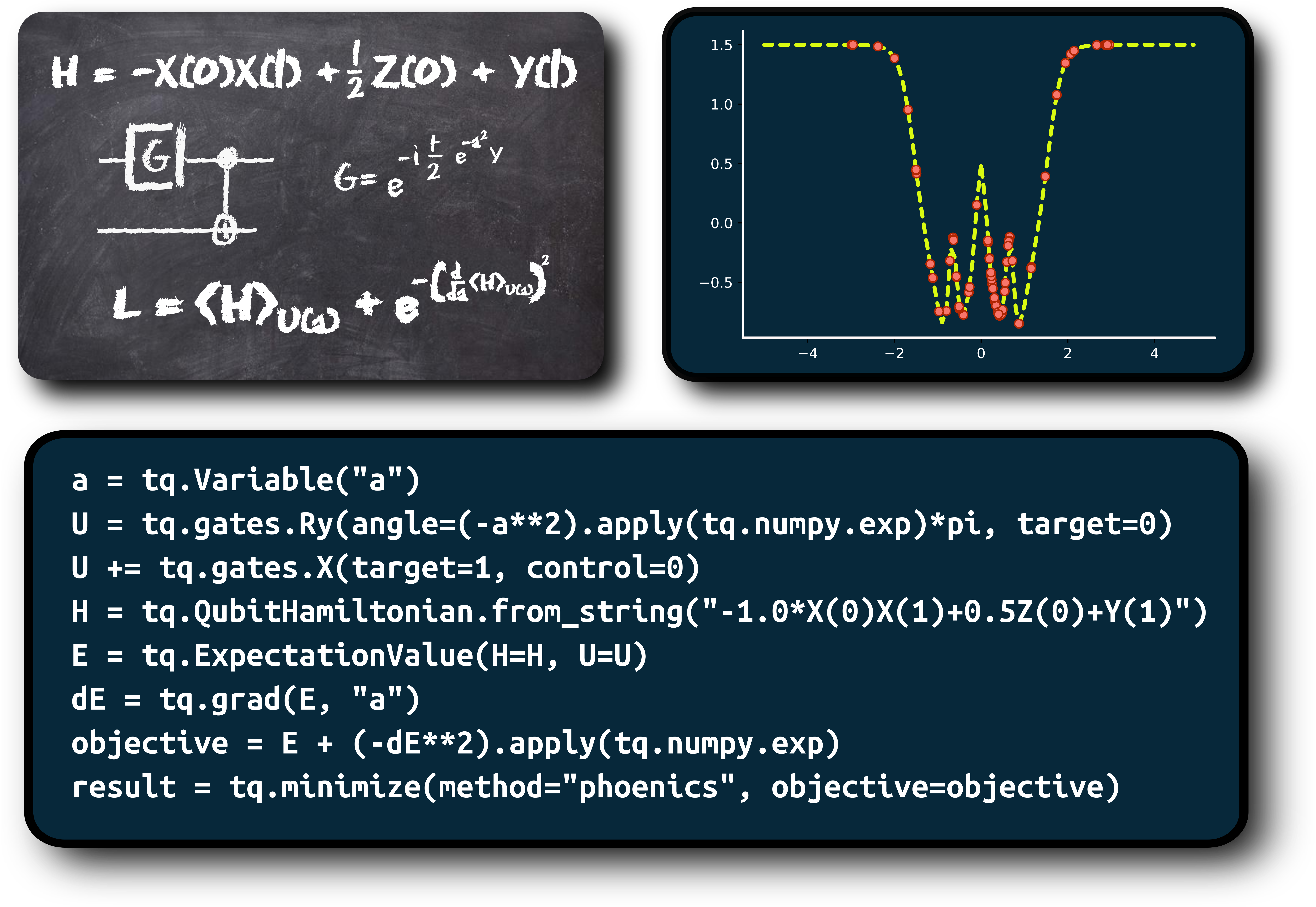
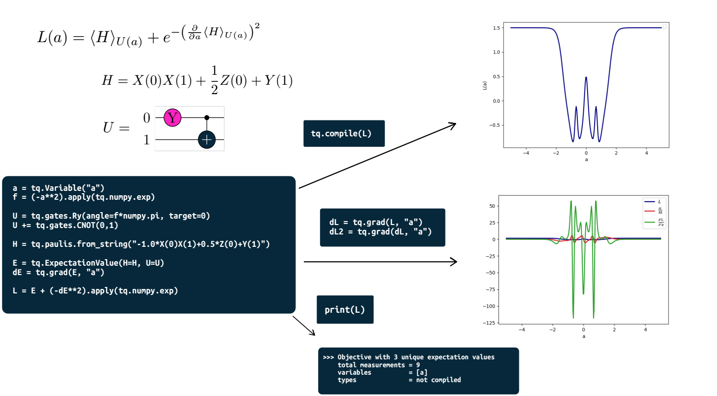
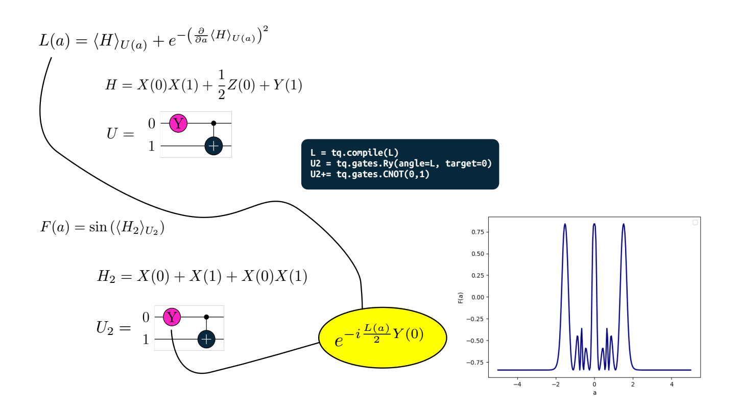
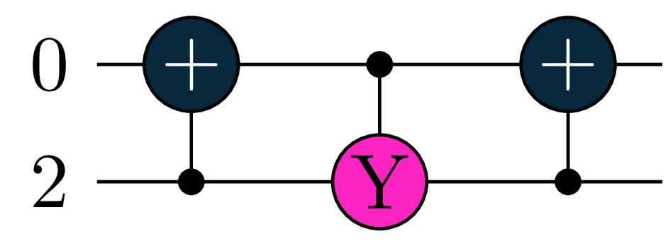
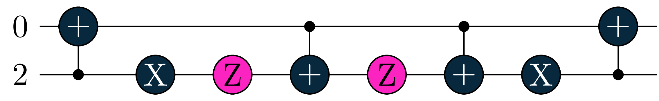
Nested example: Quantum function $L$ defines gate parameter of other quantum function $F$
Some convenient quantum gates
Standard gates in tq.gates: H, X, Y, Z, Rx, Ry, Rz, S, CNOT, SWAP
Form controlled gates with control keyword
CRy = tq.gates.Ry(angle="a", target=0, control=1)
CCRy = tq.gates.Ry(angle="a", target=0, control=[1,2])
Multi-Pauli Rotations: $e^{-i\frac{a}{2} P}$
U = tq.gates.ExpPauli(paulistring="X(0)Y(1)", angle="a", control=None)
Qubit-Excitations: $e^{-i\frac{a}{2} G}$ with e.g. $G = -i(\sigma_i^- \sigma_j^+ - \sigma_i^+ \sigma_j^-) $
U = tq.QubitExcitation(target=[i,j], angle="a", control=None)
U = tq.QubitExcitation(target=[i,j,k,l], angle="a", control=None)
U = tq.QubitExcitation(target=[i,j,k,l,m,n], angle="a", control=...)
Smart Compiler
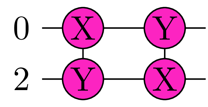
U = tq.QubitExcitation(target=[0,2], angle="a", control=None)
...
E = tq.ExpectationValue(H=H, U=U)
f = tq.compile(E, backend=...)
if backend supports MultiPauli:
 if backend supports CRy:
 otherwise:
Measurement Optimization
# full simulation is faster wihtout measurement optimization
E = tq.ExpectationValue(H=H, U=U)
# sampled runs are faster with measurement optimization
E = tq.ExpectationValue(H=H, U=U, optimize_measurements=True)
See papers by Izmaylov group (T.C. Yen, V. Verteletskyi, Z.P. Bansingh)
and the tequila tutorial
Optimizers
As tequila functions are just scalar functions, they can be minimized
result = tq.minimize(E)
final_value = result.energy
optimized_variables = result.variables
f = tq.compile(E)
final_value = f(optimized_variables)
useful
tq.show_available_optimizers()
see github tutorials on optimizers for more
Vectors, Matrices, Tensors
tq.QTensor class: Same as numpy.ndarray with abstract tequila functions
M = tq.QTensor(shape=[2,2])

M[0,0] = tq.Variable("a")**2
M[1,0] = tq.ExpectationValue(H=H, U=U)**2
M[0,1] = f**2
M[1,1] = 1.0

N = M.dot(M)

n = tq.compile(N)

evaluated_matrix = n({"a":1.0, "b":2.0, ...})
see github tutorials on QTensor for more
implemented as a qosf project (Gaurav Saxena)
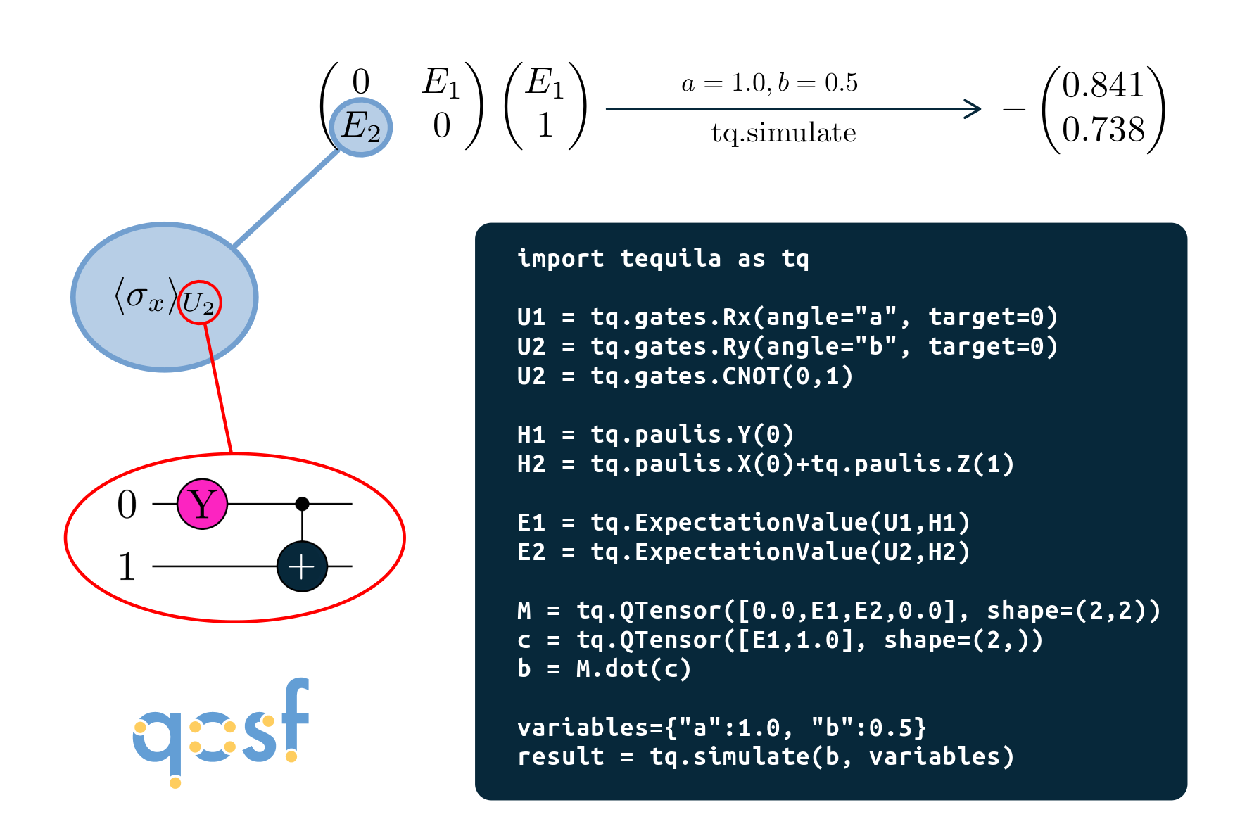
QTensor: Example
More:
- release paper: arxiv:2011.03057
- tequila on github: github.com/tequilahub/tequila
- tutorials: github.com/tequilahub/tequila-tutorials
- slide collection with research examples kottmanj.github.io/talks_and_material/
Installation:
Linux and MacOS
pip install tequila-basic
recommended to install qulacs (fastest backend)
pip install qulacs
On Windows
pip install git+https://github.com/tequilahub/tequila.git@windows
Note: Windows version is less flexible (e.g. E**2 needs to be E.apply(numpy.square) here)
See github readme for more information